RNA Velocity Geometry

FlowMap starts from a simple geometric view of RNA velocity. Each cell has a position in high-dimensional gene expression space and a velocity vector that points toward its predicted future expression state. A low-dimensional cell state embedding should preserve both pieces: where the cells are, and how they move.

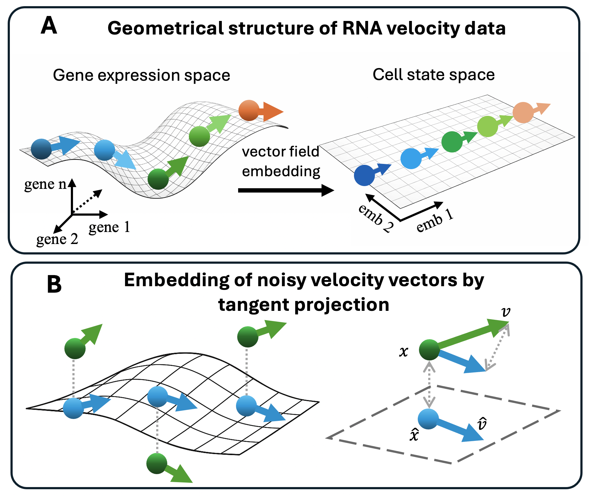
FlowMap learns a smooth relationship between a low-dimensional cell state space and the high-dimensional gene expression space, then projects velocity vectors through this local geometry.

Two Spaces

Let the low-dimensional embedding coordinate of a cell be \(z \in \mathbb{R}^d\), and its gene expression vector be \(x \in \mathbb{R}^p\), where usually \(d \ll p\).

FlowMap treats the embedding as a cell state space and learns a smooth map

\[f: \mathbb{R}^d \rightarrow \mathbb{R}^p, \qquad x \approx f(z).\]

In words, the map \(f\) tells us how a point on the embedding corresponds to a point on the gene expression manifold.

The Spline Bridge

FlowMap represents \(f\) with a smooth spline fitted from embedded cell coordinates back to gene expression space:

\[f(z) = \sum_{k=1}^{K} w_k \, \phi(\lVert z - c_k \rVert) + A z + b.\]

Here, the control points \(c_k\) define smooth local basis functions, the weights \(w_k\) reconstruct gene expression, and the affine term \(Az + b\) captures broad linear structure. This gives a smooth surface over the embedding instead of treating cells as isolated points.

Projecting Velocity

RNA velocity is observed in gene expression space as \(v = dx/dt\). To draw that velocity on the embedding, FlowMap asks: which embedded velocity \(u = dz/dt\) best explains the observed high-dimensional velocity?

The local linear approximation is given by the Jacobian of the spline:

\[\begin{split}\frac{dx}{dt} = J_f(z) \frac{dz}{dt}, \qquad J_f(z) = \begin{bmatrix} \frac{\partial f_1}{\partial z_1} & \cdots & \frac{\partial f_1}{\partial z_d} \\ \vdots & \ddots & \vdots \\ \frac{\partial f_p}{\partial z_1} & \cdots & \frac{\partial f_p}{\partial z_d} \end{bmatrix}.\end{split}\]

So the embedded velocity is obtained by projecting \(v\) onto the tangent space of the spline surface:

\[\hat{u} = \operatorname*{argmin}_{u} \left\lVert J_f(z)u - v \right\rVert^2 = \left(J_f(z)^\top J_f(z)\right)^{-1} J_f(z)^\top v.\]

For a two-dimensional embedding, this becomes:

\[\begin{split}\begin{bmatrix} \hat{u}_1 \\ \hat{u}_2 \end{bmatrix} = \left(J^\top J\right)^{-1}J^\top \begin{bmatrix} v_1 \\ v_2 \\ \vdots \\ v_p \end{bmatrix}.\end{split}\]

This is the key geometric step: FlowMap does not simply attach arrows to an embedding. It learns the local shape of the expression manifold and uses that shape to translate high-dimensional RNA velocity into cell state motion.