How to Perform Trajectory and Gene Gradient Field Analysis

Tutorials

FlowMap embedding · Velocity embedding consistency · Trajectory and gene gradients · Curvature analysis

This page shows the core FlowMap calls for fixed points, least-action paths, and gene-gradient analysis. Data loading and plotting are kept in the runnable notebook:

tutorial/larry_geometry_tutorial.ipynb

Load Data

The tutorial uses a .joblib wrapper that stores the fitted embedder with the few metadata fields and gene matrices used below. The file is not included in the GitHub repository; download it from Figshare and place it at tutorial/larry_flowmap_data.joblib before running the notebook.

Data link: Larry Data Processed with FlowMap

from flowmap.utils import load_dataset

data = load_dataset("tutorial/larry_flowmap_data.joblib")
emb = data.embedder
X_gene = data.layers["spliced"]
V_gene = data.layers["velocity"]

Fixed Points

Fixed points are places where the fitted velocity field is close to zero. FlowMap identifies candidates on a grid, smooths the speed field, and keeps low-speed regions.

from flowmap.geometry import FixedPointAnalyzer

fpa = FixedPointAnalyzer(emb)
fixed_points = fpa.identify_fixed_points(
    grid_resolution=90,
    speed_smoothing=1.2,
    speed_quantile_threshold=0.06,
)

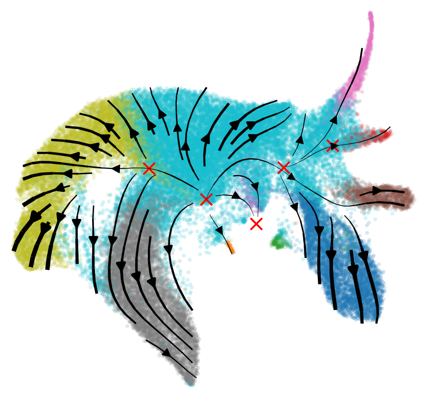
Fixed points marked on the fitted FlowMap velocity field.

Least-Action Path

A least-action path connects two points under the fitted velocity field. The main choices are the start and end positions. Here the graph initialization is built in the original feature space.

from flowmap.geometry import LagrangianPathOptimizer

start = fixed_points[0]["position"]
end = np.array([2.3, -7.6])

lap = LagrangianPathOptimizer(emb, D=1.0, lam=1e-4)
path_result = lap.fit_path(
    start=start,
    end=end,
    distance_mode="orig",
)

path = path_result["path_refined"]

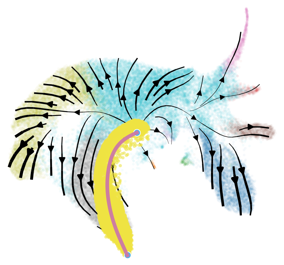
The selected path and nearby cells used for local gene-gradient analysis.

Gene-Level Splines

Gene-gradient analysis needs a spline from FlowMap coordinates back to gene expression and gene velocity.

emb.n_spline_points = None
emb.fit_gene_level_splines(
    X=X_gene,
    V=V_gene,
    dof_gene=50,
    dof_vf_gene=50,
)

Gene Gradients

The gradient analyzer computes gene-expression gradients relative to the local velocity direction. Pass only cells near the path so the Jacobian computation stays local.

from flowmap.geometry import GeneGradientAnalyzer

analyzer = GeneGradientAnalyzer(
    emb,
    cell_indices=neighbor_indices,
)

out = analyzer.compute_relative_gradients(
    neighbor_indices,
    np.arange(len(emb.gene_names)),
    weight="magnitude",
)

gradient_df = pd.DataFrame({
    "gene_idx": out["gene_indices"],
    "gene": emb.gene_names[out["gene_indices"]],
    "relative_angle": out["angles"],
    "magnitude": out["magnitudes"],
})

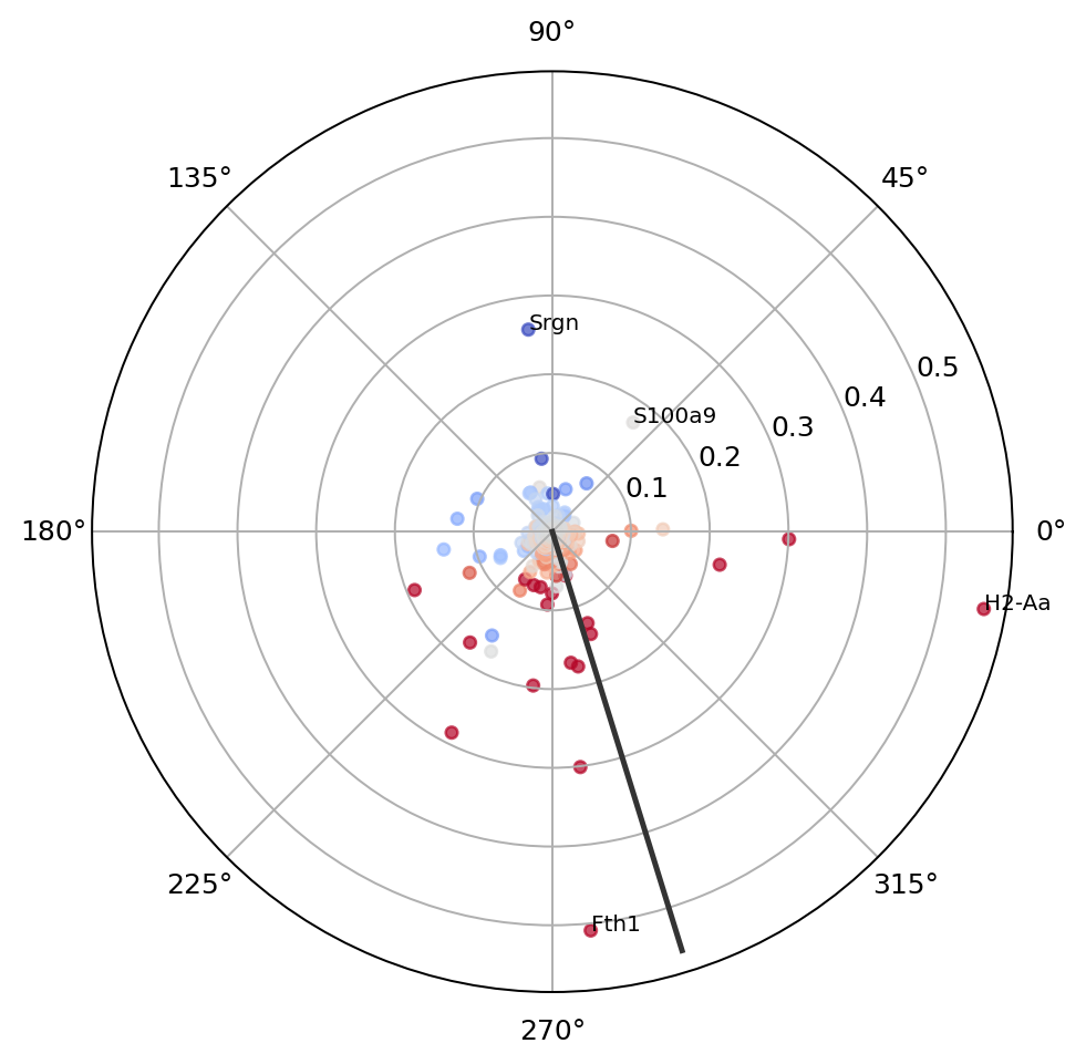
Path-local gene gradients summarized by direction and magnitude.

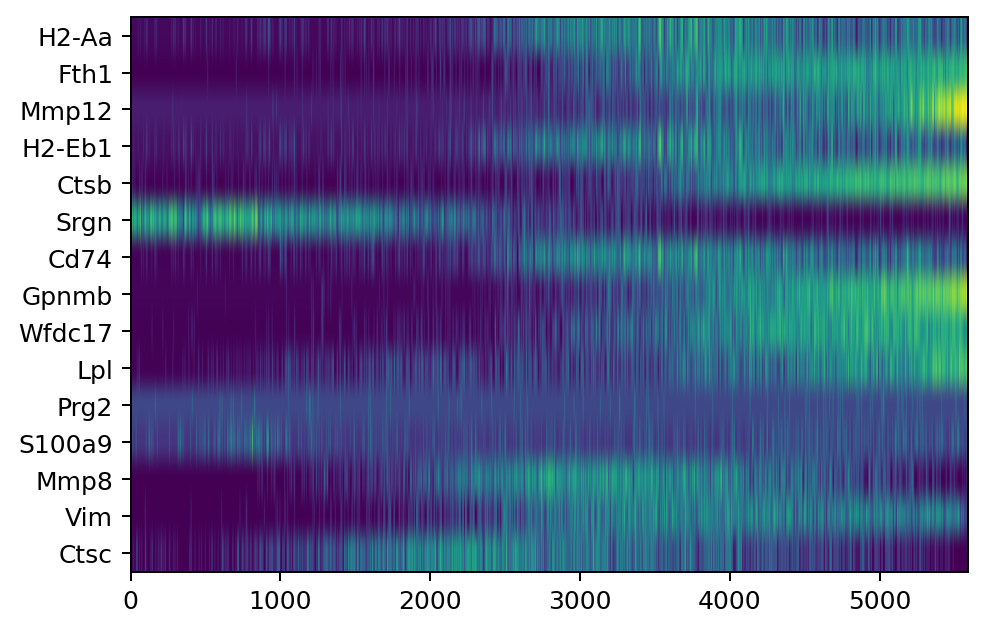
Expression of top gradient genes after ordering nearby cells along the path.

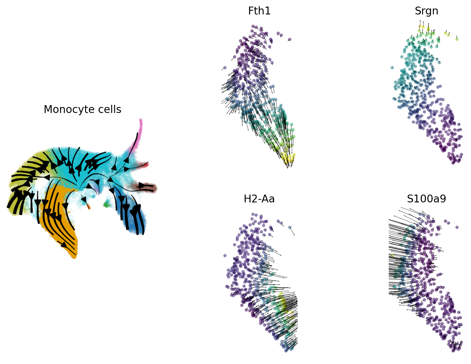
Monocyte cells on the embedding and example gene-gradient vectors for four selected genes.

The notebook contains the current plotting cells for visual inspection, but the analysis itself is the four calls above.