How to Perform FlowMap Embedding¶

Tutorials

FlowMap embedding · Velocity embedding consistency

This tutorial uses a compact cell-cycle AnnData object with 2,793 cells and 33 selected cell-cycle genes. Expression is stored in adata.X and velocity is stored in adata.layers["velocity"].

Load Data¶

import anndata as ad
import numpy as np

adata = ad.read_h5ad("example_data/cell_cycle/cell_cycle_33genes.h5ad")

X = np.asarray(adata.X, dtype=float)
V = np.asarray(adata.layers["velocity"], dtype=float)
phase = adata.obs["cell_cycle_relative_pos"].to_numpy(dtype=float)
gene_names = np.asarray(adata.var_names)

Fit FlowMap¶

from flowmap import VectorFieldEmbedder

emb = VectorFieldEmbedder(
    X,
    V,
    use_PCA=False,
    method="umap",
    dist_method="phase",
    embedding_dim=2,
    knn_k=30,
    alpha=0.5,
    embed_kwargs={"n_neighbors": 30, "min_dist": 0.3},
)

emb.fit_embedding(seed=1)
emb.fit_gene_level_splines(X=X, V=V, dof_gene=30, dof_vf_gene=30)

Plot Velocity¶

from flowmap.plot import plot_velocity_stream, plot_velocity_grid

plot_velocity_stream(
    emb.X_emb,
    spline=emb.spline_vf,
    scatter_color=phase,
    grid_size=70,
    stream_density=1.2,
    scatter_size=60,
    scatter_alpha=0.4,
    cmap="viridis",
    show_colorbar=True,
)

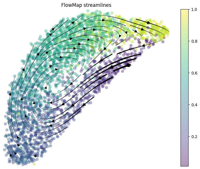
FlowMap streamline plot for cell-cycle data — Smooth streamlines show the inferred cyclic velocity field.¶

plot_velocity_grid(
    emb.X_emb,
    spline_vf=emb.spline_vf,
    scatter_color=phase,
    grid_size=25,
    scatter_size=20,
    scatter_alpha=0.35,
    arrow_scale=4.0,
    cmap="viridis",
    show_colorbar=True,
)

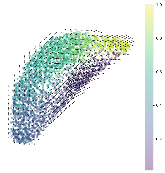
FlowMap grid velocity plot for cell-cycle data — Grid arrows summarize the smoothed velocity field across the embedding.¶

Evaluate¶

from flowmap.evaluation import SplineFitEvaluator

evaluator = SplineFitEvaluator(emb, mode="gene")
metrics = evaluator.evaluate()

print(f"Mean expression R²: {metrics['expr_r2']:.3f}")
print(f"Mean velocity R²:   {metrics['vel_r2']:.3f}")

The fitted gene-level splines give:

Mean expression R²: 0.371
Mean velocity R²:   0.214

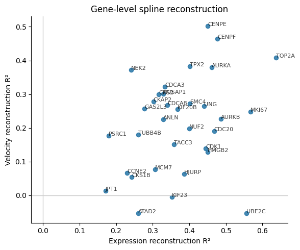
Gene-level FlowMap spline reconstruction scores — Per-gene expression and velocity reconstruction scores.¶

The runnable notebook version is available at tutorial/cell_cycle_tutorial.ipynb.