How to Perform Curvature Analysis¶

Tutorials

FlowMap embedding · Velocity embedding consistency · Trajectory and gene gradients · Curvature analysis

This page shows the core FlowMap call for curvature analysis. The runnable notebook is available at tutorial/larry_curvature_tutorial.ipynb.

Load Data¶

The Larry data object is not included in the GitHub repository; download it from Figshare and place it at tutorial/larry_flowmap_data.joblib before running the notebook.

Data link: Larry Data Processed with FlowMap

from flowmap.utils import load_dataset

data = load_dataset("tutorial/larry_flowmap_data.joblib")
emb = data.embedder

Compute Curvature¶

compute_flow_curvature evaluates the fitted manifold spline and velocity spline, then returns velocity, acceleration components, and curvature estimates.

from flowmap.geometry import compute_flow_curvature

curv = compute_flow_curvature(emb)

k_total = curv["curvature"]["total"]
k_steer = curv["curvature"]["steer"]
k_surface = curv["curvature"]["surface"]

Total Curvature¶

The total curvature combines intrinsic steering curvature and surface curvature:

\[\kappa_{\mathrm{total}} = \sqrt{ \kappa_{\mathrm{steer}}^2 + \kappa_{\mathrm{surface}}^2 }.\]

fig, ax = plt.subplots(figsize=(6, 6))
plot_velocity_stream(
    emb.X_emb,
    spline=emb.spline_vf,
    scatter_color=np.clip(k_total, None, np.percentile(k_total, 99)),
    cmap="coolwarm",
    scatter_size=10,
    scatter_alpha=0.6,
    show_colorbar=True,
    ax=ax,
)
plt.show()

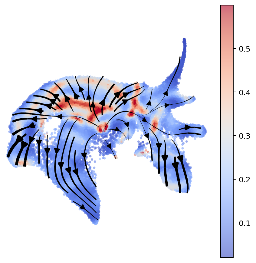
Larry FlowMap curvature on the embedding — Total curvature shown on the Larry FlowMap embedding.¶

Decomposed Curvature¶

FlowMap separates acceleration into flow, steering, and surface components. The curvature terms are acceleration magnitudes normalized by squared speed:

\[\kappa_{\mathrm{steer}} = \frac{\|A_{\mathrm{steer}}\|}{\|v\|^2}, \qquad \kappa_{\mathrm{surface}} = \frac{\|A_{\mathrm{surface}}\|}{\|v\|^2}.\]

fig, axes = plt.subplots(1, 3, figsize=(12, 4))

for ax, values, title in zip(
    axes,
    [k_total, k_steer, k_surface],
    ["total", "steer", "surface"],
):
    plot_velocity_stream(
        emb.X_emb,
        spline=emb.spline_vf,
        scatter_color=np.clip(values, None, np.percentile(values, 99)),
        cmap="coolwarm",
        scatter_size=8,
        scatter_alpha=0.6,
        ax=ax,
        title=title,
    )

plt.tight_layout()
plt.show()

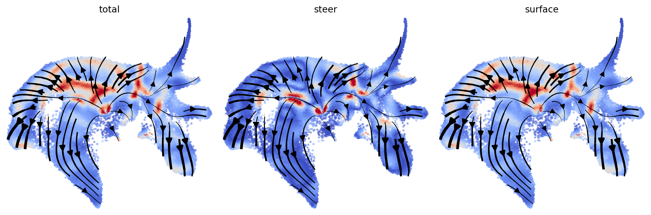
Total, steering, and surface curvature on the Larry embedding — Total, steering, and surface curvature estimates.¶

Ternary Decomposition¶

The acceleration dictionary contains flow, steer, and surface components. A ternary plot summarizes their relative contributions.

A_flow = np.linalg.norm(curv["acceleration"]["flow"], axis=1)
A_steer = np.linalg.norm(curv["acceleration"]["steer"], axis=1)
A_surface = np.linalg.norm(curv["acceleration"]["surface"], axis=1)

total = A_flow + A_steer + A_surface + 1e-12
flow_frac = A_flow / total
steer_frac = A_steer / total
surface_frac = A_surface / total

x = steer_frac + 0.5 * surface_frac
y = (np.sqrt(3) / 2) * surface_frac

fig, ax = plt.subplots(figsize=(5.8, 5.2))
ax.scatter(
    x,
    y,
    s=6,
    c=np.clip(k_total, None, np.percentile(k_total, 99)),
    cmap="coolwarm",
    alpha=0.35,
)

tri_x = [0, 1, 0.5, 0]
tri_y = [0, 0, np.sqrt(3) / 2, 0]
ax.plot(tri_x, tri_y, color="black", lw=1)
ax.text(-0.03, -0.04, "flow", ha="right", va="top")
ax.text(1.03, -0.04, "steer", ha="left", va="top")
ax.text(0.5, np.sqrt(3) / 2 + 0.04, "surface", ha="center", va="bottom")
ax.set_aspect("equal")
ax.set_axis_off()
plt.show()

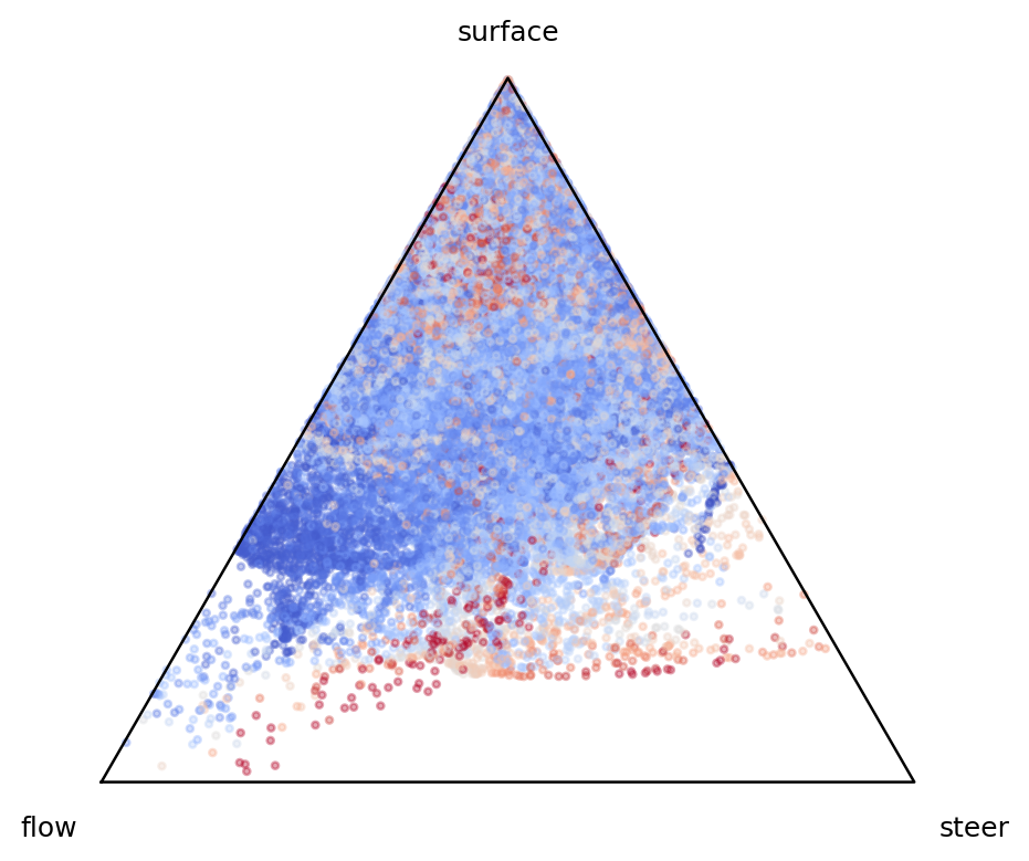
Ternary acceleration decomposition for Larry curvature — Relative flow, steering, and surface acceleration contributions.¶